You Only Accept Samples Once

We just uploaded a preprint of our research to the arXiv, titled “You Only Accept Samples Once: Fast, Self-Correcting Stochastic Variational Inference.” The work is an outcrop of the previous study we did, currently under review, trying to control the behavior of Black Box Variational Inference by regularizing it with the James-Stein estimator.

However, what we noticed in the course of testing is that, whether using Rao Blackwellization or regularization, there is a tendency for the algorithm to make large U-Turns in the middle of its run, thus losing the precious progress that it made and effectively re-starting from a less optimal position. For example, in the following figure, we show the trajectory of the objective function, called the Evidence Lower Bound (ELBO) across 1000 iterations of the original Rao-Blackwellized algorithm as well as our proposed regularization with the James-Stein (JS+) estimator.

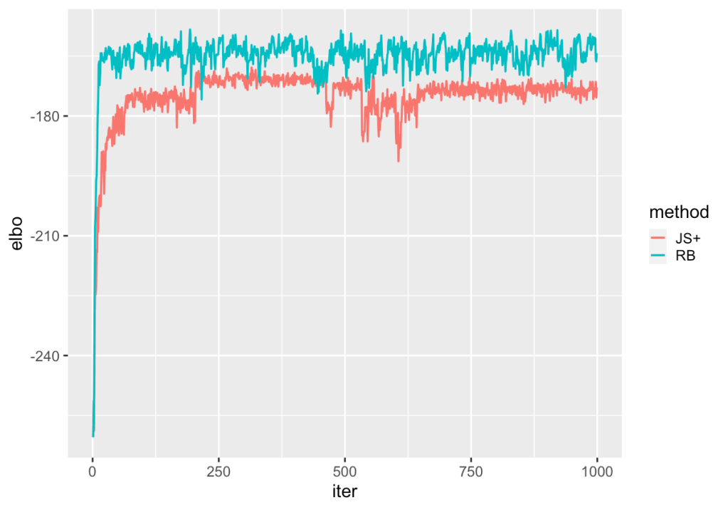
The result of this tendency to make U-Turns is the stochastic behavior of the method. Recall that the goal is to maximize the value of the ELBO, which via a common decomposition can be written as

$\mathcal{L} = \mathbb{E}[\log p(y, \theta) - \log q(\theta | \lambda)]$

for data $y$ , model parameters $\theta$ , and variational parameters $\lambda$ . Technically speaking we don’t have access to this expectation because it’s an intractable function, but we can do gradient ascent by obtaining the score function gradient estimator

$\hat\nabla_{\lambda} \mathcal{L} = \frac{1}{S} \sum^{S}_{s = 1} \nabla_{\lambda} \log q(\theta | \lambda)[\log p(y, \theta) - \log q(\theta | \lambda)]$

This estimator is very noisy and in fact if left uncontrolled has a tendency to not converge at all. The original authors of the algorithm controlled this by Rao-Blackwellization, while another paper that recently came out proposed an alternative means by applying Quasi-Monte Carlo (QMCVI) sampling such as the Halton or Scrambled Sobol sequences to directly regulate the behavior of the resulting samples. An interesting consequence of this is that the method is that it has become reasonably controlled now such that even samples of size $S = 10$ can be used (whereas the original version typically requires about $S = 500$ or as much as $S = 1000$ to $10,000$ to reach reasonable values.

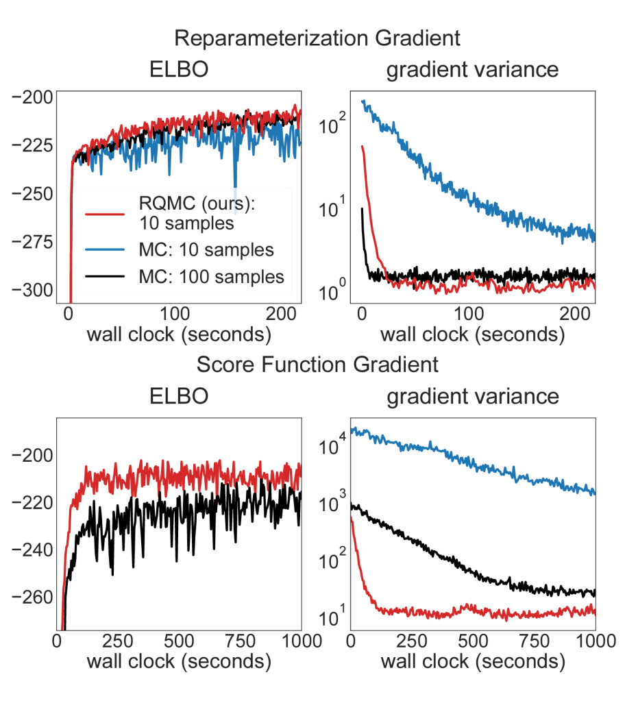
But still consider that even then, the method has a tendency to move into less optimal regions. It’s certainly become much more controlled compared to regular Monte Carlo sampling (black and blue lines in the figure). But perhaps more interesting is that the paper points to another direction of improvement for the algorithm. Using large values for the sample size $S$ yields very long computation times, since the gradient estimator has to be applied a total of $N \times S$ times, for $N$ the actual size of the data. This has been a major bottleneck in our simulation testing, since the growth in computation time from a data of size $N = 300$ to a more realistic $N = 1000$ is explosive, even with parallelization.

The QMCVI paper highlights that using a big Monte Carlo sample size may not be necessary if we can guarantee that the sample will be better behaved. More extremely, if better-behaved samples can be guaranteed, perhaps it’s even possible to use only one sample, and that’s what we investigate in the preprint. We therefore introduce YOASOVI (You Only Accept Samples Once for VI). The idea is to obtain a single sample to estimate the gradient, and then use rejection sampling to decide whether this single sample shows an improvement over the previous iteration. Specifically, if $\mathcal{L}_t$ and $\mathcal{L}_{t - 1}$ are the resulting ELBOs at the current and previous iterations, then we accept the sample at iteration $t$ with probability

$p_{accept} = \min\bigg(1, 1 + \frac{M (\mathcal{L}_{t} - \mathcal{L}_{t-1})}{\mathcal{L}_{t-1}} \bigg)$

It’s a very simple idea but one that presents a promising improvement at least based on the results of our benchmarks. Fitted on Gaussian Mixture models, YOASOVI is able to find better solutions within a few seconds, while QMCVI and BBVI both generally take about 1 to 2 minutes. The paper develops further details regarding convergence and a formalization by building the algorithm as a Metropolis-type scheme.

You Only Accept Samples Once

Share this:

Leave a comment Cancel reply